SurfSeis
MASW Software

数据的处理步骤是通过使用 SurfSeis "...\SampleData\" 子文件夹中存储的示例数据集进行演示说明。表1列出了样本数据集的所有采集参数。

图 1a—主动 MASW 法。 更多信息请参考 "主动MASW."

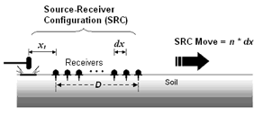
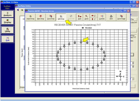
图 1b—远程被动MASW 法。更多信息请参考 "远程被动 MASW."

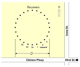
图 1c—路边被动MASW 法。更多信息请参考 "路边被动 MASW."

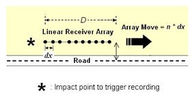
表 1—样本数据集参数摘要。

调查种类	主动 MASW	远程被动MASW	远程被动MASW	路边被动MASW
文件名	"1011.dat"-"1022.dat"	"Passive-Cross.dat"	"Passive-Circular.dat"	"4000.dat"-"4009.dat"
文件夹	"...\Active\"	"...\PassiveRemote\"	"...\PassiveRemote\"	"...\PassiveRoadside\"
调查目的	二维Vs 剖面	一维 Vs 剖面	一维 Vs 剖面	二维 Vs 剖面
数据格式	SEG-2	KGS	KGS	SEG-2
采集	24 道	48 道	24 道	48 道
震源	20-磅 锤子	交通	交通	12-磅 锤子/交通
接收器 (地震检波器)	10-Hz (尖峰耦合)	4.5-Hz (尖峰耦合)	4.5-Hz (尖峰耦合)	4.5-Hz (缆线30个 takeouts)
接收器阵列	线性 (roll along)	交叉 (x-y)	圆形	线性(roll along )
阵列尺寸(D)	23 m	115 m	115 m	35 m
接收器间隔 (dx)	1.22 m	5 m	15 m	1.2 m
震源偏移 (x1)	1.22 m	N/A	N/A	4.8 m
接收器阵列移动	1 dx (1.22 m)	0	0	4 dx (4.8 m)
采样间隔 (dt)	1 ms	4 ms	4 ms	4 ms
记录时间(T)	2 sec	20 sec	120 sec	120 sec
记录号	1011-1022	2000-2009	3000-3009	4000-4009

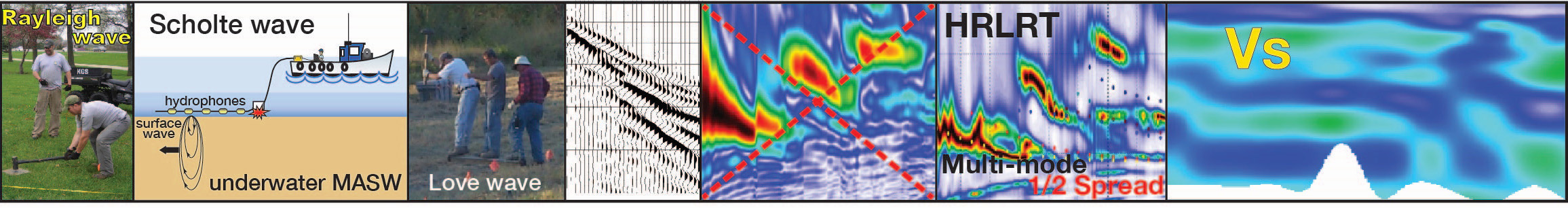
图 2中的流程图显示了使用MASW法（主动或被动）的整个过程摘要。此版本的主要更改与新功能总结如下：

1.     除了原有的主动源模块（图 1）以外，还增加了处理被动源表面波的模块。有两种不同类型的被动测量：一种称为远程被动MASW法，使用二维（2-D）接收器阵列；另一种称为路边被动MASW法，使用传统的一维线性阵列。

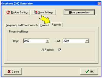
2.     更改了执行频散分析的方式，以便将先前的 '预处理-->频散-->运行-->保存' 序列分为两个单独的步骤：(1) 生成频散图像 (称为 overtone, OT) 数据和 (2) 从图像中使用鼠标辅助提取频散曲线。但是，在导入输入地震文件时，仍可以通过右键点击（而不是左键点击）分析菜单中的 'Dispersion' 按钮来访问上一个序列。

3.     增加了一种新的反演模式。这是一种通过Monte-Carlo法直接应用于频散图像（而不是频散曲线）的方法。通过随机搜索来寻找最佳匹配。通过这个方法，可以考虑最多四种频散模态。并且如果有需要，可以手动更改5层地质模型中的所有参数，以便将理论曲线与背景图像中的频散趋势进行比较。

根据许多使用SurfSeis 的MASW方法的实践者们的评论与报告， 以及他们非常有耐心的对我们这仍处于初级开发阶段的全新地理方法的软件的帮助。SurfSeis先前版本中存在的大多数（不是全部）缺陷都已经被修复。我们KGS的研究人员衷心的感谢您的耐心与意见。

图 2-- MASW 处理步骤流程图。

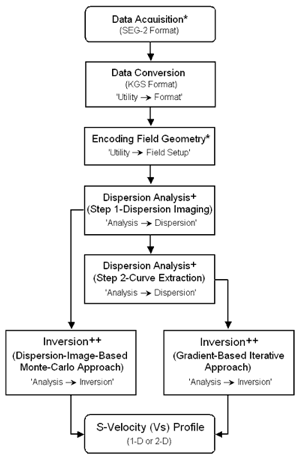
数据处理

步骤 1: 格式 (从 SEG-2 转换到 KGS 格式)

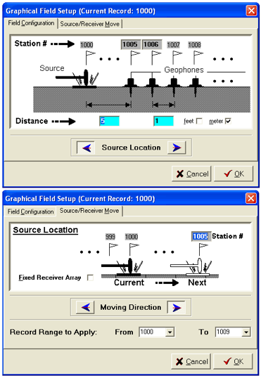
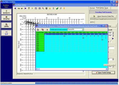
步骤 2: 场地几何编号

步骤 3: 生成频散曲线图像 (又名 overtone) 数据

步骤 4: 提取频散曲线

步骤 5: 二维Vs 剖面曲线反演 (图 5)

SurfSeis 2.0 处理步骤

场地设置 (主动调查)

以Roll-Along 模式采集的主动数据集

场地几何编号

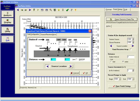
编号后的震源接收器表

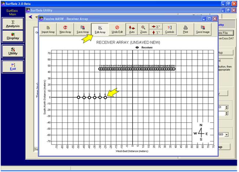
场地设置 (被动远程调查)

通过点击和拖动为每个接收器设置X-Y坐标

24道圆形阵列 (设置完成后)

48道十字阵列 (早期阶段设置)

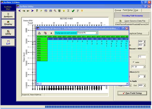
场地设置 (路边被动调查)

Roll-Along 模式采集的路边被动数据集

场地几何编号

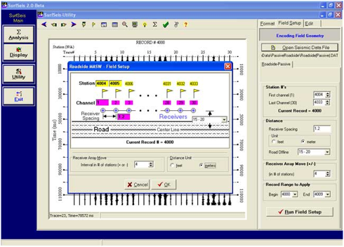
编号后的震源接收器站点表

生成频散曲线

二维波场变换生成

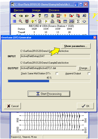
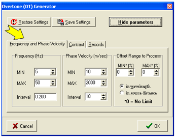
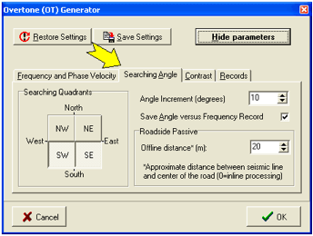
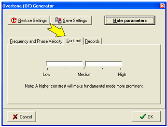
可控的处理参数

主动 (A) 和被动 (P)

只有被动 (P)

主动 (A) 和被动 (P)

主动 (A) 和被动 (P)

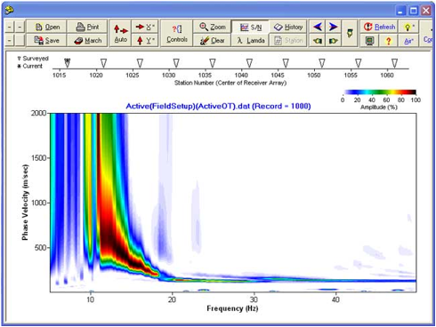
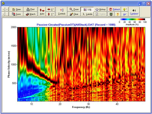
频散图像

来自主动的数据

来自远程被动的数据

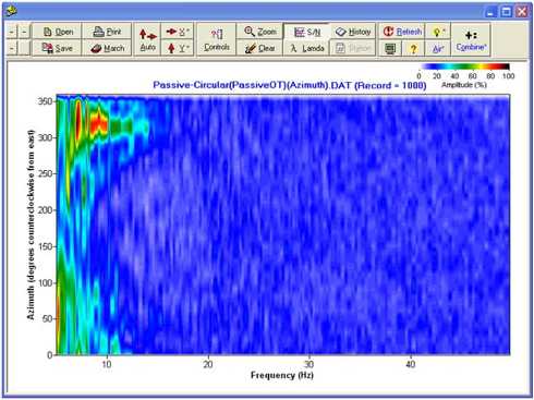
远程被动数据的方位信息

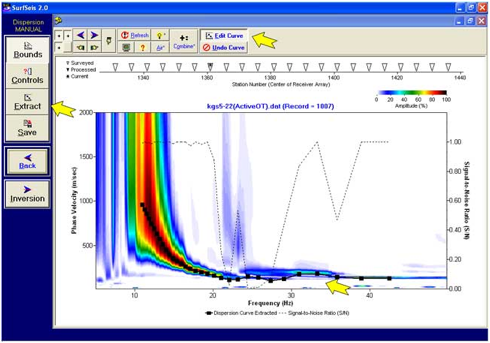
频散曲线提取

用鼠标设置相速度和频率的范围界限

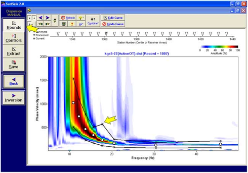
提取和编辑频散曲线

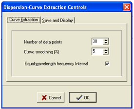
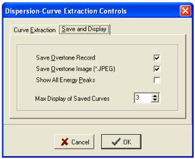
可控参数

反演提取的曲线

频散曲线的确定性反演*

*如果所有提取的频散曲线都是瑞利波基本模态，这是最快，最简单，研究最多的反演方法。当使用具有多个模态（例如，基本模态和一个或多个更高模态）的频散曲线时，由于模态解释不准确，可能会出现反演上的困难（例如，观测曲线和计算曲线之间的拟合差，均方根误差较高） (Ivanov et al., 2010) 。

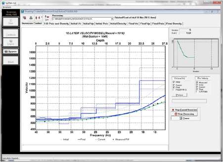
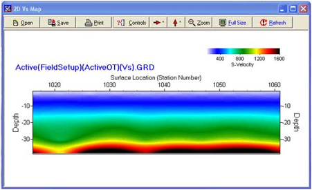
来自反演的二维Vs剖面

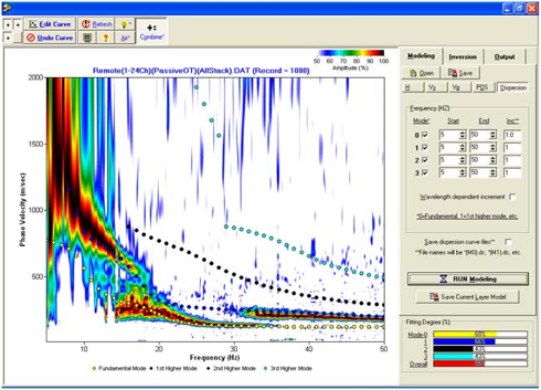
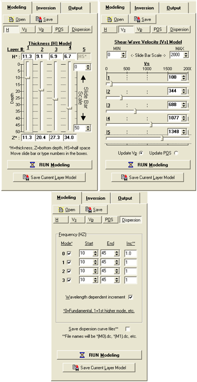
频散曲线图像的建模与随机反演

此工具允许用户手动更改模型参数，计算多达4个瑞利波模态，并将其绘制在频散曲线图像上进行比较。

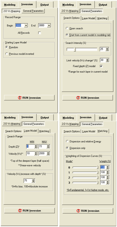
Monte-Carlo 法的二维Vs剖面自动反演

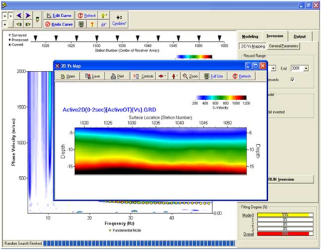
随机反演 (控制)

Monte-Carlo (一种随机) 反演法，可以通过随机改变模型参数，计算频散曲线的点，并将它们与频散曲线图像上的振幅进行比较来实现。这种方法可能非常耗时，但它时一个有用的研究工具。

请注意，不用的模型可以计算来自不同模态的频散曲线点，这些点与频散曲线图像的拟合度相同。因此，在模式解释时选择此解决方案具有重要意义。

同样，在进行任何类型的反演建模时，请记住

1.     频散曲线图像可能不同，具体取决于

a.     震源的偏移量和测线的尺寸，

b.     频散曲线图像的计算方法与参数。

2.     使用HRLRT 进行频散曲线成像时，对分离不同模态，以及理解在频散曲线图像上不同趋势的可能性会非常有用 (Ivanov et al., 2010).

正向建模部分

反演部分

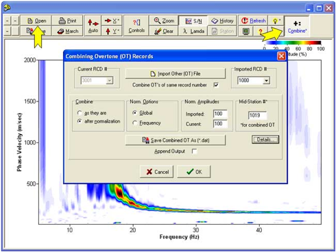
结合主动与被动频散

增加频率 (深度) 范围...

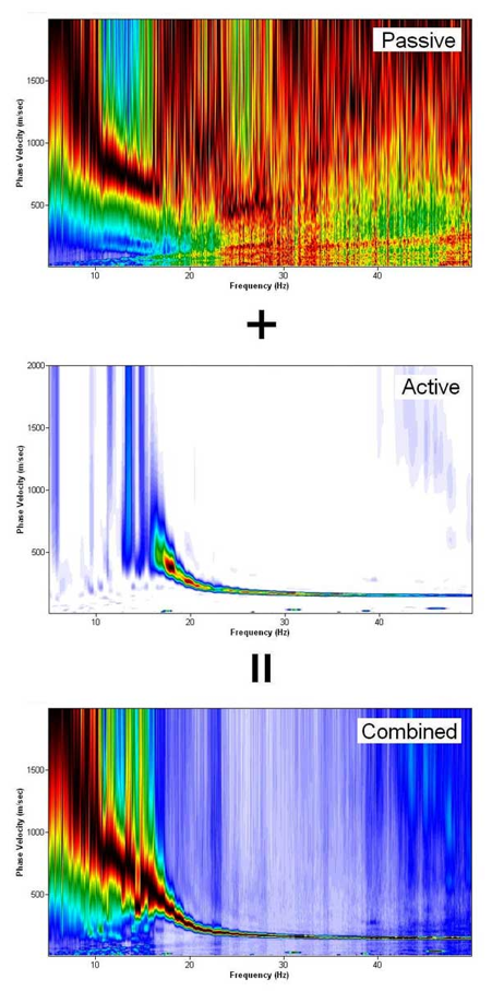
帮助模态识别...

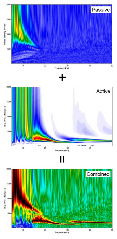
打开主动 (或被动) 图像，然后将被动 (或主动) 图像组合在一起

参考文献

Ivanov, J., R. D. Miller, and G. Tsoflias, 2008, Some Practical Aspects of MASW Analysis and Processing: Symposium on the Application of Geophysics to Engineering and Environmental Problems, 21, 1186-1198.

Ivanov, J., R. D. Miller, J. Xia, and S. Peterie, 2010, Multi-mode inversion of multi-channel analysis of surface waves (MASW) dispersion curves and high-resolution linear radon transform (HRLRT): 80th Annual International Meeting, SEG, Technical Program Expanded Abstracts, 29, 1902-1907.

Luo, Y. H., J. H. Xia, R. D. Miller, Y. X. Xu, J. P. Liu, and Q. S. Liu, 2009, Rayleigh-wave mode separation by high-resolution linear Radon transform: Geophysical Journal International, 179, 254-264.

Matheron, G., 1967, Kriging or Polynomial Interpolation Procedures--a Contribution to Polemics in Mathematical Geology: Canadian Mining and Metallurgical Bulletin, v. 60, no. 665, p. 33-58.

Miller, R. D., T. S. Anderson, J. Ivanov, J. C. Davis, R. Olea, C. Park, D. W. Steeples, M. L. Moran, and J. Xia, 2003, 3‐D characterization of seismic properties at the smart weapons test range, YPG: 73rd Annual International Meeting, SEG, Technical Program Expanded Abstracts, 22, 1195-1198.

Miller, R. D., J. Xia, C. B. Park, and J. M. Ivanov, 1999, Multichannel analysis of surface waves to map bedrock: The Leading Edge, 18, 1392–1396.

Olea, R. A., 1974, Optimal Contour Mapping Using Universal Kriging: Journal of Geophysical Research, 79, 695-702.

Park, C. B., and R. D. Miller, 2008, Roadside passive multichannel analysis of surface waves (MASW): Journal of Environmental and Engineering Geophysics, 13, 1-11.

Park, C. B., R. D. Miller, D. Laflen, C. Neb, J. Ivanov, B. Bennett, and R. Huggins, 2004, Imaging dispersion curves of passive surface waves: 74th Annual International Meeting, SEG, Expanded Abstracts, 23, 1357-1360.

Park, C. B., R. D. Miller, N. Ryden, J. Xia, and J. Ivanov, 2005, Combined use of active and passive surface waves: Journal of Environmental and Engineering Geophysics, 10, 323-334.

Park, C. B., R. D. Miller, and J. Xia, 1998, Imaging dispersion curves of surface waves on multi-channel record 68th Annual International Meeting, SEG, Expanded Abstracts, 1377-1380.

Park, C. B., R. D. Miller, and J. H. Xia, 1999, Multichannel analysis of surface waves: Geophysics, 64, 800-808.

Song, Y. Y., J. P. Castagna, R. A. Black, and R. W. Knapp, 1989, Sensitivity of near‐surface shear‐wave velocity determination from rayleigh and love waves: 59th Annual International Meeting, SEG, Expanded Abstracts, 8, 509-512.

Xia, J. H., R. D. Miller, and C. B. Park, 1999, Estimation of near-surface shear-wave velocity by inversion of Rayleigh waves: Geophysics, 64, 691-700.

Xia, J. H., Y. X. Xu, and R. D. Miller, 2007, Generating an image of dispersive energy by frequency decomposition and slant stacking: Pure and Applied Geophysics, 164, 941-956.